The Lightning Network holds the promise of enabling nearly instantaneous settlements for Bitcoin payments. However, achieving this goal in a sovereign way presents substantial technical challenges, primarily due to the opacity of channel balances, which is inherent to the design of the network. In this blog post, we will delve into the workings of pathfinding (or payment planning in a wider sense) within the Lightning Network, with a specific focus on its implementation in LND. We discuss current techniques for making payments more reliable and aim to provide a detailed examination of how LND determines channel preferences and explore recent developments, including the introduction of a new probability estimator.

Payment Prerequisites

Payments on the Lightning Network can feel almost instantaneous, but there is a lot going on under the hood while a payment is in flight. In order to carry out a multi-hop payment on the Lightning Network, we broadly have to fulfill two prerequisites:

1. we need to receive an invoice to know the recipient of the payment
2. we need to have a fully synchronized view of the network topology to have detailed knowledge about how to route from the sender to the receiver

The first prerequisite is simply fulfilled by some out-of-band communication between sender and receiver at the time of payment. The second prerequisite, however, is more involved.

Lightning Network nodes obtain the network topology information (also known as the graph) via peer to peer gossip messages. These messages include essential metadata like information about channel capacities (indirectly obtained via channel ids) and HTLC (hash timelocked contracts) constraints like the minimal or maximal HTLC size. They also include whether a channel is marked disabled, and the fee charged by each router to forward the payment. Though they are transmitted individually, multiple channels may coexist between two peers advertising different channel constraints. When pathfinding, the payer's node will synthesize these parallel channels into a unified edge in order to anticipate worst case constraints (e.g. taking the largest fee rate or time lock delta). The routing node actually forwarding the payment down these parallel channels though is free to choose any of them to forward the payment, which is called non-strict forwarding. This is an important first step to improve route reliability.

Payments can be made reliable as well by involving good routing nodes that provide the liquidity in places where it's needed, combined with smart pathfinding algorithms that can find the liquidity. Ideally, a planned payment is successful on the first attempt based on past payment experience and any signals the gossip graph provides. However, routers are not perfectly efficient in their actions, which is why channel failures due to lacking liquidity are expected to happen. Delivering a payment thus involves a trial and error loop. Moreover, a Lightning payment can be conducted not only along a single route but can be split into multiple parts.

Payment Loop in LND

This section briefly outlines the life cycle of a payment in LND. To kick off the payment process, a user looking to send a payment provides the invoice generated by the receiver to the payment system, which amends the network graph with additional information like optional hop hints to know how to reach a destination via the "last mile". Payment planning also needs to know about the amount to be sent as well as the protocol features the destination supports (e.g. do they support multipart payments?), which are included in the invoice as well. At this point we enter the payment loop, which is displayed in the following diagram:

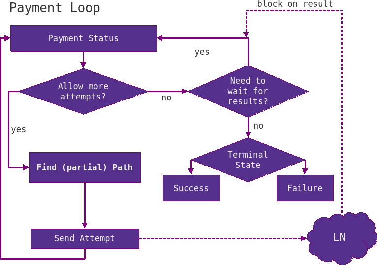
We first check the payment status, which signals an initiated payment, but no attempts have been sent yet and we are thus allowed to send new HTLC attempts. We then compute a path for the total amount (details on pathfinding are described later) and send the payment along the selected outgoing channel and path. At this point, we have given up control about the payment's fate whereby the payment is now in-flight. We don't allow for new attempts, because the total payment amount is already pending and we need to wait for our peer to reply with either a settlement or a failure.

The most common failure case is a temporary channel failure, which indicates that some hop along the route lacked liquidity. Other cases include the next node being down or that insufficient fees were added. This is valuable information we can employ to improve our next route selection. We learn about the successful and unsuccessful parts of the route by evaluating from which node the error originated from. This information is recorded in so-called "mission control" that keeps track of the successful/unsuccessful amounts and their timestamps.

The loop continues with newly selected routes, taking into account the liquidity information provided by mission control until the payment either succeeds or the estimated success probability drops below a certain threshold (more on success probabilities later). This is when we enter multi part payments. In order to increase the success probability for individual attempts again, we have to split the payment amount into smaller pieces. Payment splitting strategies are a work in progress and payment reliability can be further enhanced by adding redundant overpayments to the protocol, see here for early conceptual work. LND currently employs a divide and conquer scheme, dividing the remaining payment amount into halves. These parts are then sent out concurrently and waited on their simultaneous settlement or timeout.

Pathfinding

The details of how suitable routes are evaluated and found were left out so far. Given a payment amount and destination, how can we select a path that is reliable and cheap? It turns out that the design space for this problem is large and this represents a trade-off as well.

Due to multipart payments, mathematically speaking the fundamental problem to deliver a Lightning payment is rather to find a flow (a combination of multiple individual paths) with the desired total low opportunity and fee costs instead of finding a single path. However, LND currently employs a divide and conquer splitting strategy mentioned in the previous section to find a flow iteratively, which boils back down again to finding single paths using Dijkstra's shortest path algorithm.

Dijkstra's algorithm is a breadth-first-search algorithm with a priority queue that keeps track of "distances" to nodes in the network, much like wave fronts exploring a maze flooded with water. The distances play an important role and they are evaluated as a combination of ingredients. They are expressed in units of fees accumulated along the path, but they should be regarded as virtual fees we minimize for in order to trade off the real routing fees with certain properties of the route that enter as virtual fee heuristics.

It is this aspect of pathfinding that has the largest degree of freedom for research. To be more concrete, besides the base fee and fee rate, the HTLC lock time and other costs to favor or penalize shorter or longer routes, node response times, node reputation or physical distances may enter. All these factors can influence the time it takes for a payment to arrive.

Payment times are strongly influenced by being able to estimate whether a route will be successful or not. In the Lightning Network, we are confronted with hidden channel balances, an intended privacy and scalability trade-off. Not knowing channel balances makes it difficult to plan payments ahead of time. So how can we factor in the opportunity cost a failing payment represents to us? How can we define a threshold below which we stop sending the total amount and start splitting it into smaller chunks?

Probability/Fee Trade-Off

The answer to the two preceding questions lies in path success probability estimation. The question of how we can trade off fees against the opportunity cost can be answered by the following arguments. Given path success probabilities $P_A$ and $P_B$ for two paths $A$ and $B$ (with the same amount) with associated routing fees ($F_A$ and $F_B$), we can evaluate the expected costs for two scenarios: $A$ is tried first then $B$, or $B$ is tried first then $A$. We associate each failure with a constant opportunity cost $O$ we forfeit with an unsuccessful attempt. This opportunity cost does not really materialize in terms of fees, but we have to pay for it by waiting, which is why this is also called attempt cost. The two scenarios are:

• Expected cost for A then B:

• Expected cost for B then A:

Comparing the costs, say $F_{AB} < F_{BA}$, after some algebra leads to an inequality of

This indicates how we can compare the virtual fees of two paths, namely by multiplication of $O$ with the inverse of the path success probability as $F_O(P) = O / P$.

We highlight that LND works with total path probabilities in the Dijkstra priority queue. An alternative would be to express virtual probability costs in terms of their negative log hop probabilities $P_i$. The latter would be advantageous should one's algorithm require a per-hop weight instead of a term that applies for the whole path, by employing the logarithm's product splitting property to result in individual hop terms with $\log(1/P) = \log\left(1/\prod_i^{\text{hops}}P_i\right) = -\sum_i^{\text{hops}}\log(P_i)$. Both approaches make the total path cost dependent on the product of individual hop probabilities $P = \prod_i^{\text{hops}} P_i$.

In LND today, the opportunity cost is composed of a constant and proportional term depending on amount $x$ to send:

The cost $F_O(P)$ encodes the statement: how much more would we rather pay in order to know with certainty that a payment succeeds via a previously tried path versus exploring another unknown but potentially cheaper path. The larger $O$ is chosen via its two parameters, the stronger we tend to the former action, valuing our time more. This trade-off is exposed in LND's settings routerrpc.attemptcost and routerrpc.attemtpcostppm. Additionally, at payment time, this can be tuned via a time preference parameter in QueryRoutes and SendPaymentV2.

This gives us the final path distance metric used in LND today as follows

noting that routing fees ($F_\mathrm{fees}$) take fees of fees into account and that the total HTLC lock time is converted to a virtual fee $F_\mathrm{locktime},$ which is proportional to the payment amount $x$ by a conversion factor. We stress here again that with the term $F_O(P)$ we can weigh the last term against the others, expressing our preference of fees over reliability.

Probability Estimation: a priori Model

Path probabilities have long been taken into account in LND, they were introduced in 2019. In the next section, we want to discuss how probabilities are estimated. An early model for hop success probabilities that saw several rounds of improvements is called a priori (Latin for from the earlier - independent of any experience), which is a simple yet effective default estimator in LND. The concept relies on defining a default hop success probability, the a priori probability (apriori.hopprob), which is assumed to be constant for any untried channel and amount. It is currently defined with a default value of 60%, slightly biasing towards more assumed successes than failures. The value of 60% for the a priori value is just an assumption and not meant to represent the real network situation, it rather acts as a way to provide a base opportunity cost for unknown channels which can be lowered by previous successful attempts to bias more towards those channels. This gives us the very simple prior hop probability $P(x) = 60\%$, with $x$ the amount to send.

Recall that mission control records previous successes and failures for given amounts on a per hop basis, which we can use to make informed decisions to deviate from the a priori probability. The a priori estimator assigns high hop probability for amounts lower or equal than a previous success amount $x_\text{success}$, giving us the conditional probability

Should a hop have failed to route with amount $x_\text{fail}$, it is assigned a penalty by lowering its success probability to zero, thereby creating infinite cost with the 1/P term, leading to avoidance of the hop. In order to give the channel another chance in the future, the a priori probability is recovered after some exponential backoff time (apriori.penaltyhalflife, which defaults to one hour). This is in contrast to the previous success probability, which remains static at a value of 95%. This encodes the specification that successful hops should be retried until proven otherwise by experiencing a failure.

To give an example, we compare three routes A, B, and C each with a given fee rate and success probability. We ignore base fees, fees of fees, lock time, and the base attempt cost to simplify the discussion. Route A with routing fees 0 ppm (parts per million = 0.000001) has failed previously and now has a success probability $P_A=10\%$. Route B with 50 ppm is untried with $P_B=60\%$, and route C with 100 ppm was successfully paid over before with $P_C=95\%$. We assume an attempt cost of 1000 ppm and a payment amount of 100 ksat.

The total virtual fees accumulate to $F_\text{path}(x) = x \cdot \mathrm{fee\_rate} + x \cdot \mathrm{attempt\_cost\_rate} / P_\text{path}$ with

Comparing all routes, we see that we would retry route C due to its low virtual fees, knowing it will succeed with some certainty over trying out a new route B that would be cheaper by 42 sat, but comes with uncertainty. Route A is neglected due to its high opportunity cost.

The a priori model described so far has a drawback, namely that the a priori probability is independent of the amount and channel capacity. Intuitively, one may agree that sending a smaller amount should have a higher chance of success than sending the whole channel capacity. This issue was addressed in a recent PR. The a priori probability becomes capacity dependent by multiplication with a capacity factor

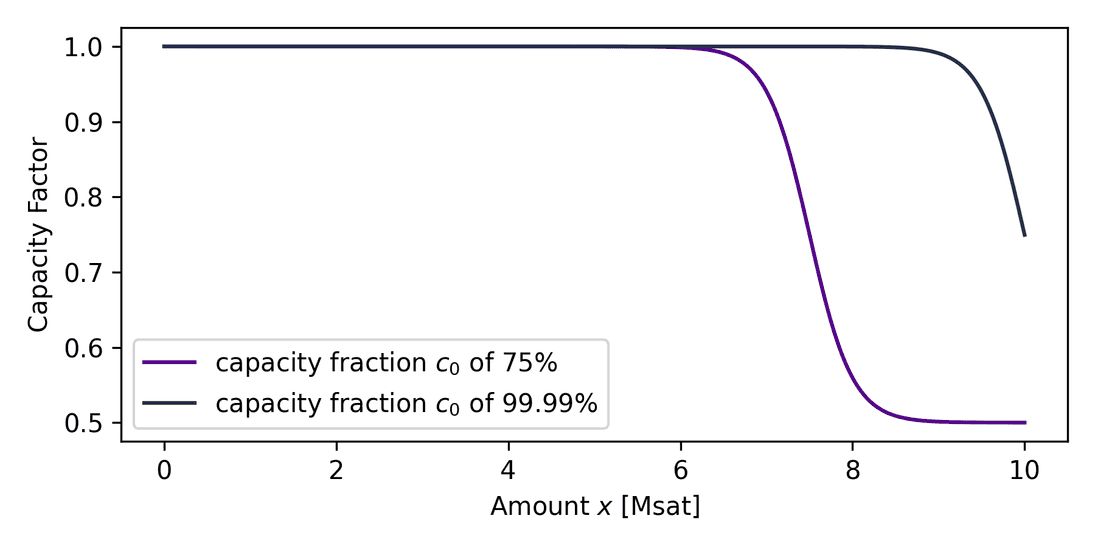
This function is close to unity for small amounts and reduces the probability strongly when the amount is close to a defined fraction $c_0(c) = c/c_0$ of the capacity, controlled by the routerrpc.apriori.capacityfraction setting. A smearing variable $s_0(c) = c/s_0$ influences how quickly the function drops (interactive demo). Multiplication of the a priori probability with this factor will thus disfavor channel exhaustion.

Conclusion

In the initial part of the pathfinding blog series, we presented fundamental concepts of pathfinding, starting with the payment loop and its relation to route computation. We delved into the elements essential for path selection and addressed the challenge of balancing reliability and fees by concentrating on a simple representation of payment success probability. Our exploration led us to refine the success probability by taking the capacity into account, serving as a segue to replacing the simple model with a more advanced one - a model that employs a more rigorous mathematical description. This post contained insights and ideas from several people who influenced the development of pathfinding in lnd, a non-exhaustive list is Joost Jager, Roasbeef, Rene Pickhardt, and yyforyongyu. A huge thank you to those contributors! Stay tuned for Part 2 where we’ll explore bimodal pathfinding, probability estimates, and gossip signals.